Section 1. Introduction

Suppose we want to estimate the average height of adults in a city. We randomly sample people and use their average height as our estimate. We have already learned that, as the sample size tends to infinity, the sample average converges to the true average. In practice, however, we only have a finite sample, say, 10 people, so our estimate will generally have some error. How large can this error be?

The tricky part is that our sample is random. Consider a simple example: 99% of adults are 170 cm tall and 1% are 200 cm tall. The citywide average is therefore 170.3 cm. If we independently sample 10 people, we could happen to select 10 unusually tall people. To cover every possible sample, we would need an error bound of 29.7 cm, which is too large to be useful.

But in most samples, the error is much smaller. In fact, we will usually sample only people who are 170 cm tall, giving an error of just 0.3 cm. The 29.7 cm bound is so large because it must also cover unusual samples. As a result, it tells us little about the error we typically encounter.

One way to address this is to allow a small chance that the bound fails. In this example, the sample contains at most one unusually tall person with probability greater than 99.5%. Whenever this happens, the estimation error is at most 2.7 cm. By allowing a failure probability below 0.5%, we reduce the error bound from 29.7 cm to 2.7 cm.

This is the kind of guarantee concentration inequalities provide: with a finite sample, the estimation error stays below a specified threshold with high probability. To obtain general bounds that apply to a wide range of distributions, we work with limited information, such as the range or variance, rather than specifying the full distribution.

Section 2. Where It All Begins

How can we obtain such a general bound? It all starts with a simple idea: continuing with our height example, by counting how many people are at least a given height, we can work out how large the average must at least be.

Consider our sample of 10 people: eight are 170 cm tall and two are 200 cm tall. Their heights, in cm, are

The average height is (8 × 170 + 2 × 200)/10 = 176 cm. We can also learn about this average by counting how many people reach a given height.

For example, all 10 people are at least 170 cm tall. Their total height must therefore be at least 10 × 170 = 1700 cm. Dividing by 10 tells us that the average must be at least 170 × (10/10) = 170 cm.

Now choose 200 cm instead. Two people reach this height, so these two alone contribute at least 2 × 200 = 400 cm to the total. The other heights cannot be negative, so the total must be at least 400 cm. Dividing by 10 tells us that the average must be at least 200 × (2/10) = 40 cm.

More generally, choose a height t and split everyone into two groups: those below t and those at least t tall. Each group contributes its fraction of people multiplied by its average height:

The first group’s average is at least 0. The second group’s average is at least t. Replacing each average by its lower bound gives

Notice that, when bounding the first group’s contribution, we implicitly used a property of heights: they are nonnegative. Of course, this holds in practice. In a more general setting, this assumption matters: if the first group contained negative values, its contribution could be negative rather than at least zero.

The reasoning in the example above extends to a general result. For any nonnegative random variable X with a finite mean, and any t > 0,

Dividing both sides by t > 0 gives

The rearrangement in Eq. (2) gives us a new interpretation: knowing only the mean of a nonnegative random variable lets us control how often large values occur. The probability that X reaches or exceeds t is at most $\frac{𝔼\left[X\right]}{t}$.

Section 3. One Step Further

Eq. (2), derived from the example above, is the well-known Markov’s inequality. We will see in this part that it is very useful. But recall our original question: how can we bound the error when we use the average height of 10 people to estimate the citywide average? Markov’s inequality does not directly answer this question.

Don’t worry, we can use Markov’s inequality to bound the error by applying it to the squared deviation from the mean. For a random variable X with finite variance, define $Y={(X-𝔼[X\left]\right)}^2$. Applying Markov’s inequality to Y gives, for any t > 0,

Whether X is positive or negative, Y is always nonnegative because it is a square. We therefore no longer need X itself to be nonnegative. This is Chebyshev’s inequality.

Here, |X − 𝔼[X]| measures how far X is from its mean. Eq. (3) says that the probability of this distance being at least t is no larger than Var(X)/t². At the same threshold t, a smaller variance gives a smaller probability bound. Equivalently, X stays within t of its mean with probability at least 1 − Var(X)/t².

In our height example, the citywide average is 170.3 cm, and the variance of an individual’s height is 8.91 cm². For 10 independent samples, the sample average has variance 8.91/10 = 0.891 cm². Chebyshev’s inequality tells us that the probability of an estimation error of at least 3 cm is at most 0.891/3² = 9.9%. In other words, our estimate is within 3 cm of the citywide average with probability at least 90.1%.

Markov’s inequality is often called a tail bound because it bounds the probability that X exceeds a threshold (Figure 3). Chebyshev’s inequality is a concentration inequality because it bounds the probability that X deviates from its mean by at least t, telling us how closely X is concentrated around its mean (Figure 4). We can now derive more tail bounds and concentration inequalities using similar methods.

Section 4. Controlling Tails through Moments

In Section 2, we derived Markov’s inequality under the assumption that X is nonnegative. Let us summarize it formally.

Now apply Markov’s inequality to $Y=X^k$ for nonnegative X. Using $t^k$ as the threshold, we obtain

This means that, besides the mean, which is the first-order moment (i.e., k = 1), we can also use moments of other orders to control the tail probability.

Remember what a moment is? We can think of moments as a series of summaries of a distribution. The most familiar is the first-order moment, $𝔼[X]$, which is the mean. The second-order central moment, $𝔼[{(X-\mu )}^2]$, is the variance, where μ = 𝔼[X].

For nonnegative X, higher powers give large values more weight relative to small values. If large values occur often, they make the moment large. Heuristically, knowing that a moment is small limits how often large values can occur, so we can use it to control the tail probability.

However, using a higher-order moment does not necessarily give a tighter tail bound: the denominator $t^k$ changes too. To find the tightest bound among the available moment bounds, we compare the different orders and take the infimum:

This is also called a higher-order moment bound.

Section 5. From Tail Bounds to Concentration Inequalities

In Section 3, we applied Markov’s inequality to $Y={(X-𝔼[X])}^2$ to obtain Chebyshev’s inequality. We can also apply Eq. (5) to $Y=|X-𝔼[X]|$ and take k = 2 to get the same result. The absolute value ensures that Y is nonnegative. Therefore, unlike the variable in Markov’s inequality, X itself does not need to be nonnegative. Let us summarize it below.

Note that, with only variance information and no further assumptions on the distribution, Chebyshev’s inequality is sharp in general. This means we cannot replace it with a smaller bound that holds for every such distribution. To see why, we only need to find a distribution for which equality holds.

Here is an example. For any given t > 0, choose any mean μ and any p ∈ (0, 1], and let

Then 𝔼[X] = μ, and

Thus, for every threshold, there is a distribution that attains equality. We do not require the same distribution to attain equality at every threshold.

Applying Eq. (5) to $Y=|X-𝔼[X]|$ and substituting k = 2 gives Chebyshev’s inequality. We choose this order because the second central moment is the variance, a familiar and widely used measure. However, k = 2 does not necessarily give the tightest bound for a particular distribution and threshold. This does not contradict Chebyshev’s inequality being sharp, because the two statements use different information. Here is an explanation.

Chebyshev’s inequality is sharp when we know only the variance: we cannot give a smaller bound that works for every distribution with that variance. But if we also know moments of other orders, we have more information than just the variance. These additional moments may give a tighter bound than k = 2. We can therefore compare the available orders:

Here, μ = 𝔼[X], and the infimum is over positive integer orders with finite absolute moments.

For example, let X take −1 and 1 with equal probability, and choose t = 2. Its mean is zero, and both its second and fourth moments equal 1. Using the second moment gives an upper bound of 1/2² = 1/4. Using the fourth moment gives a smaller upper bound of 1/2⁴ = 1/16. The fourth moment gives us additional information that can improve the bound.

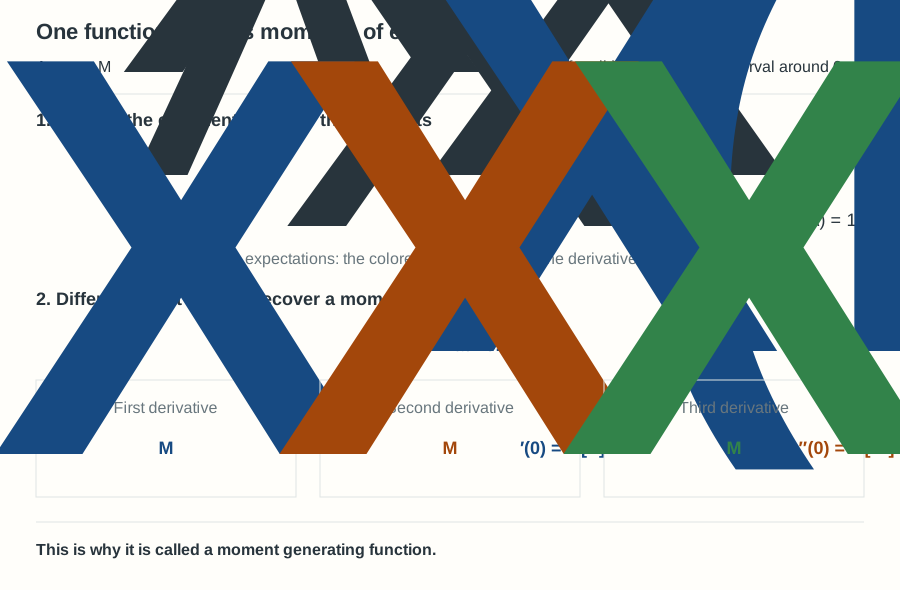
So far, we have used moments to control concentration. We can now extend this approach by using a moment generating function (MGF). Intuitively, it packages moments of all orders into one function, written as $M_X(\lambda )=𝔼[e^{\lambda X}]$. We consider values of λ for which this expectation is finite. When the MGF is finite in an open interval around zero, its power series contains all the moments, and differentiating it at zero recovers each one. Figure 6 illustrates this relationship.

Let μ = 𝔼[X]. We now apply Markov’s inequality to $Y=e^{\lambda (X-\mu )}$, using $e^{\lambda t}$ as the threshold. For λ > 0, the exponential is increasing, so X − μ ≥ t is equivalent to Y ≥ e^λt. Also, Y is always positive, even when X − μ is negative. Whenever the expectation below is finite, we obtain

This holds for every positive λ for which the expectation is finite. Just as we compared different moment orders, we can compare different values of λ and take the infimum. Writing the ratio as an exponential gives the Chernoff bound, summarized below.

As with Generalized Markov’s Inequality, we have a parameter to choose. Here, λ acts as a tuning parameter, much like the moment order k. We choose the value that makes the right-hand side smallest, giving the tightest bound available from this approach. The best value may depend on t and the MGF.

Notice that Eq. (10) bounds X − μ rather than |X − μ|. We applied Markov’s inequality to e^λ(X−μ), not e^λ|X−μ|, so it controls only the upper tail. To obtain a two-sided concentration bound, we also apply the same argument to μ − X. When the relevant expectations are finite, this gives

Let B₊(t) denote the upper-tail bound in Eq. (10), and B₋(t) the lower-tail bound in Eq. (11). A deviation of at least t from the mean occurs in either the upper tail or the lower tail. Adding their probability bounds gives

The two bounds need not be equal. If the same MGF upper bound applies to both signs of λ (which is quite common, as we will see later), both tails can use the same bound B(t), and we obtain

Let us summarize the connections. Each bound starts from Markov’s inequality and chooses a different nonnegative variable Y. Figure 7 shows what we substitute, the conditions we need, and the bound we obtain.